Annoying join behavior in QGIS

Today I stumbled across something I wouldn’t exactly consider a bug, but at least some rather unintuitive and annoying behavior in QGIS when performing table joins.

I did something very mundane: joining a Postgres table of spatial data to another Postgres table of attribute data. The normal way to do this (for me) is as follows:

  1. Open the spatial table using Layer > Add Layer > Add PostGIS Layers...
  2. Open the attribute table the same way (1 & 2 can be loaded in one go)
  3. Join the tables in the spatial table’s Properties dialog.

For that last step I decided to join the two tables (plr is the spatial table here, while mss has the attributes) using the field plr_id, which exists in both tables and only once on each side (hence a plain vanilla 1:1 join).

Add vector join dialog window in QGIS 2.8

Add vector join dialog window in QGIS 2.8

That works perfectly fine, except that somehow the order of the joined fields appears to get messed up:

QGIS attirbute table with erroneously shifted field contents

QGIS attirbute table with erroneously shifted field contents

Some research revealed that this seems to be a problem caused by identical field names in the two joined tables other than the join field itself. In my case the aforementioned plr_id was used to join the two tables, but in addition both tables also had a field gid, as can be seen in the following screenshot on the left:
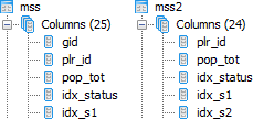
Table design in pgAdmin: original table including field gid on the left, fixed table without (unnecessesary) field gid on the right

Table design in pgAdmin: original table including field gid on the left, fixed table without (unnecessesary) field gid on the right

Removing this field gid from the attribute table mss was no problem, since the 1:1 relation to the spatial data uses the key plr_id anyways. As can be seen in the screenshot above on the right, the new table mss2 is identical to mss, only without the field gid. And lo-and-behold – joining this attribute table to the spatial table plr in QGIS works flawlessly now:

QGIS attirbute table with correct field contents

QGIS attirbute table with correct field contents

This problem had already been identified in QGIS 2.0 in late 2013, and has been marked as fixed in the meantime. Removing fields with identical names in the two tables is one – admittedly rather radical way – to solve circumvent the issue. Another, more intuitive way would be to choose a meaningful table prefix in the Add vector join dialog which can be seen in the first image above. As you can see I checked the Custom field name prefix checkbox but left the field empty. I prefer this, since it keeps my field names nice and tidy, but in cases where homonymous fields exist in the two tables you will run into trouble – hence entering a prefix here would be a nice and easy fix for this issue.

Everything described above was performed on QGIS 2.8.1-Wien (64bit) on a Windows 7 machine and PostgreSQL 9.1.16 on a 64bit Ubuntu 4.6.3 server (PostGIS 1.5.3).

The Power of Vectorization in R

I have always been a great fan and avid user of databases. They’re just so versatile, efficient, easy to use, … I found this to be true for all kinds of data, small and large, high-dimensional and low-dimensional, spatial, temporal, you name it. It was only very recently that my data seemed to have outgrown my PostgreSQL database. Not so much in size, but rather in performance.

Continue reading →

Using Tokyo

In the introduction to the UN HABITAT report State of the World’s Cities 2012/2013: Prosperity of Cities it is written:

“As the world moves into the urban age, the dynamism and intense vitality of cities become even more prominent. A fresh future is taking shape, with urban areas around the world becoming not just the dominant form of habitat for humankind, but also the engine-rooms of human development as a whole. This ongoing evolution can be seen as yet another assertion, albeit on a larger scale, of the time-honoured role of cities as centres of prosperity. In the 21st as in much earlier centuries, people congregate in cities to realize aspirations and dreams, fulfil needs and turn ideas into realities.”
(United Nations 2012, v)

I could not agree more, and this is one of the reasons that I was captivated by cities from an early age, long before I started my academic career – or even had an idea of what an academic career is, for that matter. Cities interest me, cities fascinate me, and cities defined me. Having lived in Munich, Frankfurt, and Tokyo, and having visited many other amazing specimen worldwide has definitely had an impact on me and taught me many things. Studying cities is never boring and continues to surprise and astonish me on a regular basis.

Continue reading →

Batch-Loading and Merging Shape Files Into PostGIS

Today I was faced with the task of having to load a massive amount of shape files into my PostGIS database. The data in question is the Advanced Digital Road Map Database (ADF) (拡張版全国デジタル道路地図データベース) by Sumitomo Electric System Solutions Co., Ltd. (住友電工システムソリューション株式会社). It contains very detailed information (spatial and attributive) about the road network of all Japan and is thereby quite heavy.

Therefore, it was split into a plethora of files using the following naming schema: mmmmmm_ttt.shp, where mmmmmm represents a six-digit mesh code and ttt represents a 2- to 3-digit thematic code. The mesh code is a result of the data being split spatially into small, rectangular chunks. It follows a simple logic, whereby bigger mesh units (represented by the first four digits) are further subdivided into smaller units (represented by the last two digits). It took only a small amount of time to figure out this naming schema and filter the files that would be necessary for my analysis.

Basically I wanted to merge the shape files into PostGIS tables divided by their topic (i.e. road nodes, road links, additional attribute information, etc.). So I had to find a way to batch import the shape files into PostGIS and merge them at the same time. Yet, since the node IDs were only unique within each mesh unit (i.e. shape file), I also had to find a way to incorporate the mesh codes themselves into the data, so I could later on create my own ID schema for the nodes, based on the mesh code and the original node ID (e.g. mmmmmmnnnnn, where mmmmmm represents a six-digit mesh code and nnnnn represents the original 5-digit node ID).

Continue reading →

Working With Non-Unicode Data in Python

Being a researcher in Japan means I often have to work with Japanese data. While generally data is data is data, there are some peculiarities I came across that seem to be related to the fact that those data are about and produced in Japan.

Firstly there is the way they are delivered. I’m no so much talking about deliveries on “hard media” such as CD-ROMs and DVDs being snail-mailed, even though this seems to be the major way of obtaining data until this day. Luckily I’m embedded in an ecosystem of research institutions and university laboratories that engage in joint research projects and thereby share the necessary datasets online using portal websites. I’d especially like to mention the JoRAS portal of the Center for Spatial Information Science (CSIS) at the University of Tokyo (東京大学) here, since their stock is quite extensive and they are always open for collaboration inquiries.

Secondly there is the fact that, not very surprising, Japanese datasets often contains Japanese data. By this I’m not referring to the fact that this data is dealing with information about Japan, but to the fact that it is making use of Japanese script. This introduces some technical difficulties, which I would like to elucidate in this article.

Continue reading →